Pinhole: a falling ball demo
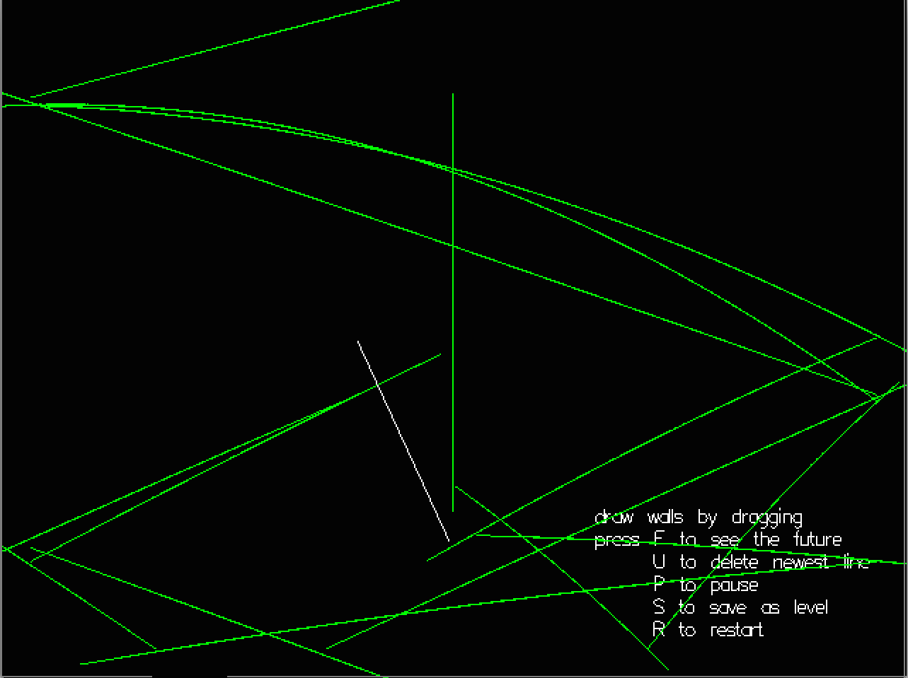
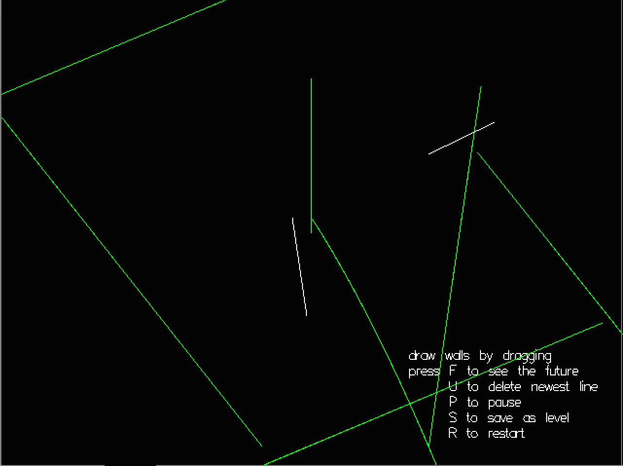
Hover your mouse over this screenshot to *see into the future*
At Hacker School last year (I was part of the winter 2013 batch), I spent a few days making a falling ball game/demo (source on GitHub). I've neglected to write it up and package it until now. It's pretty simple, but it's got one really cool feature that I wanted to show off: you can ~~see into the future~~.
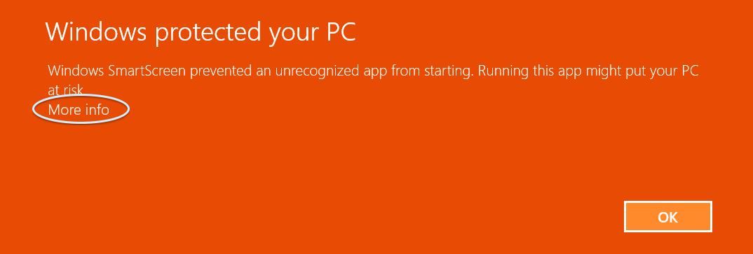
You can download Pinhole for Mac OS X and Windows.1 On Windows, you may see some warnings from Chrome or Windows that the file isn't commonly downloaded; you can bypass Chrome's warning and bypass Windows' warning (step one, step two). E-mail me if you have problems.
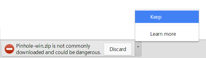
Playing around
The green line segment in each ghost ball represents the translational velocity vector of the center of the ball.2
I want to play around a bit with the premises here. What if we jack up the sampling resolution?
Increasing the sampling resolution to get a smooth curve
One cool thing I didn't even realize is that the density of ghosts in some place tells you how slowly the ball is going in that place. If the ball moves through somewhere quickly, the ghosts will be sparser there.
There's also some kind of resonance thing going on with the crosses inside the ghost balls.
Huh, there's also something interesting there with the green velocity segments. They were individual indicators before, but now they've connected into a smooth line. What happens if we take away the ghost balls so we just see that green line?
Stripping away the balls
Notice that now we're literally just doing some operations to a curve.3
Our vocabulary has changed from 'a ball and walls and falling down' into 'a curve and some constraints on the curve'. Well, with this new vocabulary, the rules this demo follows are just arbitrary. They don't need to fit the metaphor of a ball rolling into a hole at the bottom of the screen. Let's play around with them.
If we increase the normal force parameter from 1.10 to 1.5,4 we get something a lot bouncier:
Bouncier
And if we go even further up, to 5, gravity hardly even shows up. I like to think of the ball as an ideal particle at this point:
Like gas particles
Sure, we start running into little imperfections:
-
the ball has a nonzero radius, so the green line (at its center) is significantly offset from the walls our particle hits (at its edge)
-
if you make your normal force too large then the line doesn't even appear, because the ball goes offscreen too fast (because we're just sampling where the ball is, we're not actually looking at a continuous function)
-
for the same reason, sometimes the ball overshoots a wall and gets forced back (as you can see)
-
the green line has little wedges wherever it makes a turn, showing the last velocity of the ball before it turns; it's really supposed to be a velocity indicator, not a point representing the ball's position
But now that we have the idea, we at least know we can move in that direction and fix those imperfections, if we think this is a cool thing to pursue.
Technical details
The other really cool feature isn't a feature at all; it's a particular tool I chose. Half of the reason I built this thing was so that I could play around with the Haskell programming language.
It makes this cool foresight trick easier than you'd think!
I'll go through a similar progression to the one in the previous section, but this time with examples from the demo's code modules PlayState, Step, and especially Draw. I want to explain how this thing works and why my tool choice makes it natural to do.
Let's start by defining the type PlayState: a PlayState is a data structure representing the current state of the world of the demo. If we wrote down the PlayState on a piece of paper, stopped the demo, and then typed what we wrote down back into the program somehow and restarted it using that PlayState, it should keep going, exactly the same as before.
data PlayState = PlayState {
      level :: Level -- walls, other stuff built into level

    , balls :: [Ball] -- balls' (right now just 1) positions, radii, velocities

    , drawnWalls :: [Wall] -- walls the user has drawn themselves
                           -- in this session

    , docState :: DocState -- should we show the documentation on screen?
                           -- how long has it been up there?

    , drawing :: DrawState -- is the user drawing a line right now?
                           -- what are its endpoints?

    , future :: Bool -- does the user want to see the future?

    , paused :: Bool -- is the game paused?
    } deriving (Show)
At any given time, we have a PlayState object (record) with these fields.5 Each frame, the Gloss library (the library I'm using for graphics and input and everything else) sends our PlayState object (called pl below) to the stepPlay function, which returns a new PlayState for the new frame.
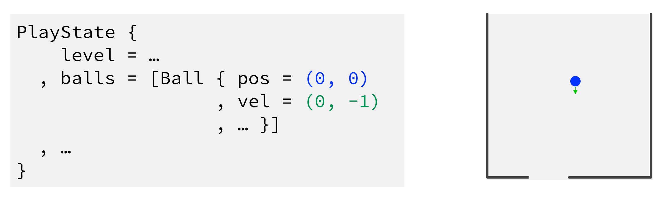
A PlayState object (excerpt on left) represents a situation like the one on the right (not to scale) (enlarge). The blue dot is the ball's position; the green arrow is its velocity. These are both representations of the same information, and I'll use both to visualize PlayState objects for the rest of the post.
We might, for instance, give stepPlay a PlayState with the ball at the top of the screen, and it might give us back a new PlayState where the ball's now a little bit further down because of gravity. Here's the code:
stepPlay :: Float -> PlayState -> PlayState
stepPlay dt pl@(PlayState { level = l, balls = bs,
                            drawnWalls = ws, drawing = dwg }) =
    pl { balls = let ws' = walls l ++ case dwg of
                                        Drawing dw -> dw:ws
                                        NotDrawing -> ws in
                 map (\b -> foldr collideWB (stepBall dt b) ws') bs }
Okay, so we step the ball forward (adding its velocity to its position, making gravity act on its velocity) and collide the ball with the level's walls (plus drawn walls, plus the wall the user's currently drawing, if they are in fact drawing a wall).
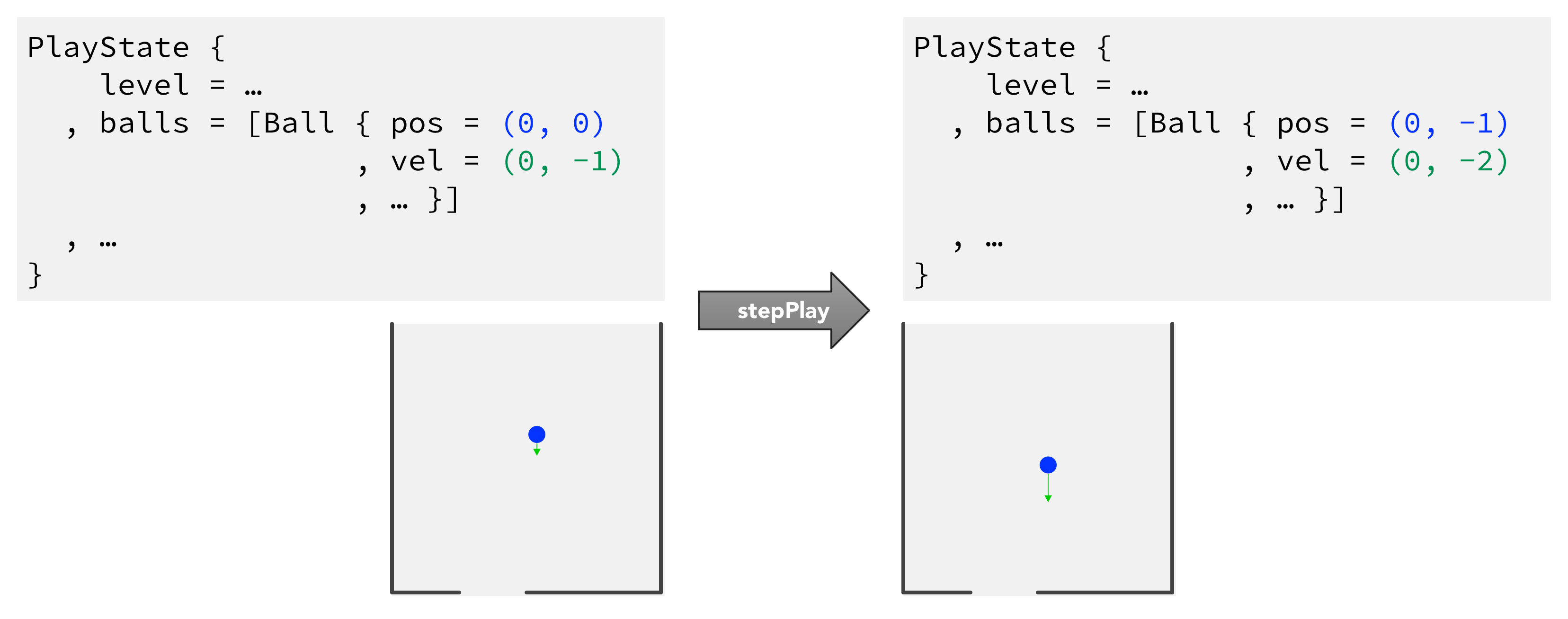
Moving one step forward by passing a PlayState (left) into stepPlay and getting a new PlayState (right) (enlarge)
So how do we see into the future? To actually make our demo in Gloss display stuff on the screen, we make a function drawPlay that turns a PlayState into a Picture (a type in Gloss that you can make out of various shapes). That Picture object basically contains information like "draw a white circle of radius 10 at coordinates (5, 5), and a gray line from (0, 0) to (11, 1)...".
drawPlay :: PlayState -> Picture
drawPlay pl | future pl = pictures [ drawFutures pl, drawPlayState pl ]
            | otherwise = drawPlayState pl
drawPlay doesn't do any drawing itself; it dispatches that to these functions drawPlayState and drawFutures. It basically just checks whether the user wants to see into the future (future pl).
If they do, then we put the Picture we get from drawFutures pl on top of the one from drawPlayState pl; if they don't, then we only display drawPlayState pl, since the user doesn't want to see the future.
drawPlayState does the 'real' drawing, rendering the ball as a circle and walls as lines and combining all that stuff gleaned from our PlayState into one giant Picture.
![drawPlayState turns numbers (left) into actual circles and lines (right)[^abstract] (enlarge)](images/drawPlayState.png)
drawPlayState turns numbers (left) into actual circles and lines (right)[^abstract] (enlarge)
More interesting to us is drawFutures, which renders our view into the future.
drawFutures :: PlayState -> Picture
drawFutures = pictures . take 100 . map (drawFutureBalls 50000) .
              filter ((== 0) . (`mod` 15) . fst) .
              zip [0..] . iterate (stepPlay 0)
I've expressed drawFutures in 'point-free style', as a composition of functions, instead of giving its argument (a PlayState) a name (in the earlier functions, I used pl). (Point-free style is kind of controversial; some of the extreme cases are unreadable. I think this case is pretty nice, but you might disagree.)
That means we've got a pipeline of functions here; we send the PlayState through these functions, and at the end we wind up with a Picture of the future6. Read it backwards:
-
iterate (stepPlay 0): theiteratefunction iteratesstepPlay 0over the PlayState that was passed intodrawFutures, and returns an infinite list of iterations.If we name the PlayState we've got right now
pl, this step returns a list like[pl, stepPlay 0 pl, stepPlay 0 (stepPlay 0 pl)...], meaning[the PlayState right now,the PlayState next frame,the PlayState the frame after that...].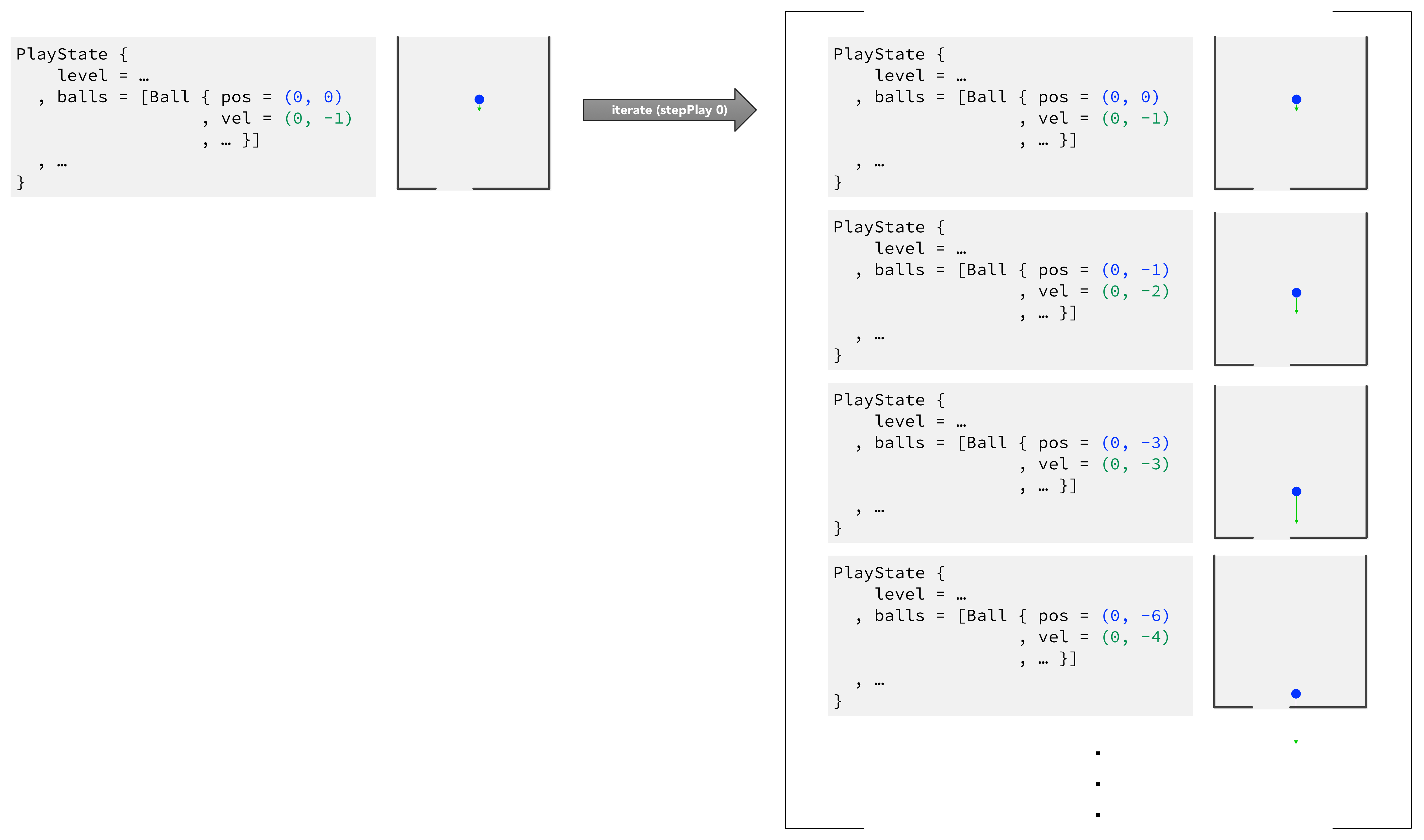
Iterating our current PlayState into an infinite list of future PlayStates (enlarge)
This step is the key step!
iterategives us access to the entire future of the world. This trick is only possible at all becausestepPlayis a pure function that gives you a new PlayState, rather than just modifying properties of an existing PlayState. We can peek into the future easily, just by looking into this giant (in fact, infinite) list, without having to go out of our way to store that temporary data somewhere separate from our 'real' PlayState.Now we'll just filter and transform all those snapshots of the future into a picture of ghosts.
-
zip [0..]: we usezipto tag each PlayState in our list of future PlayStates with an index, so we have[(0,the PlayState right now), (1,the PlayState next frame), (2,the PlayState the frame after that)...]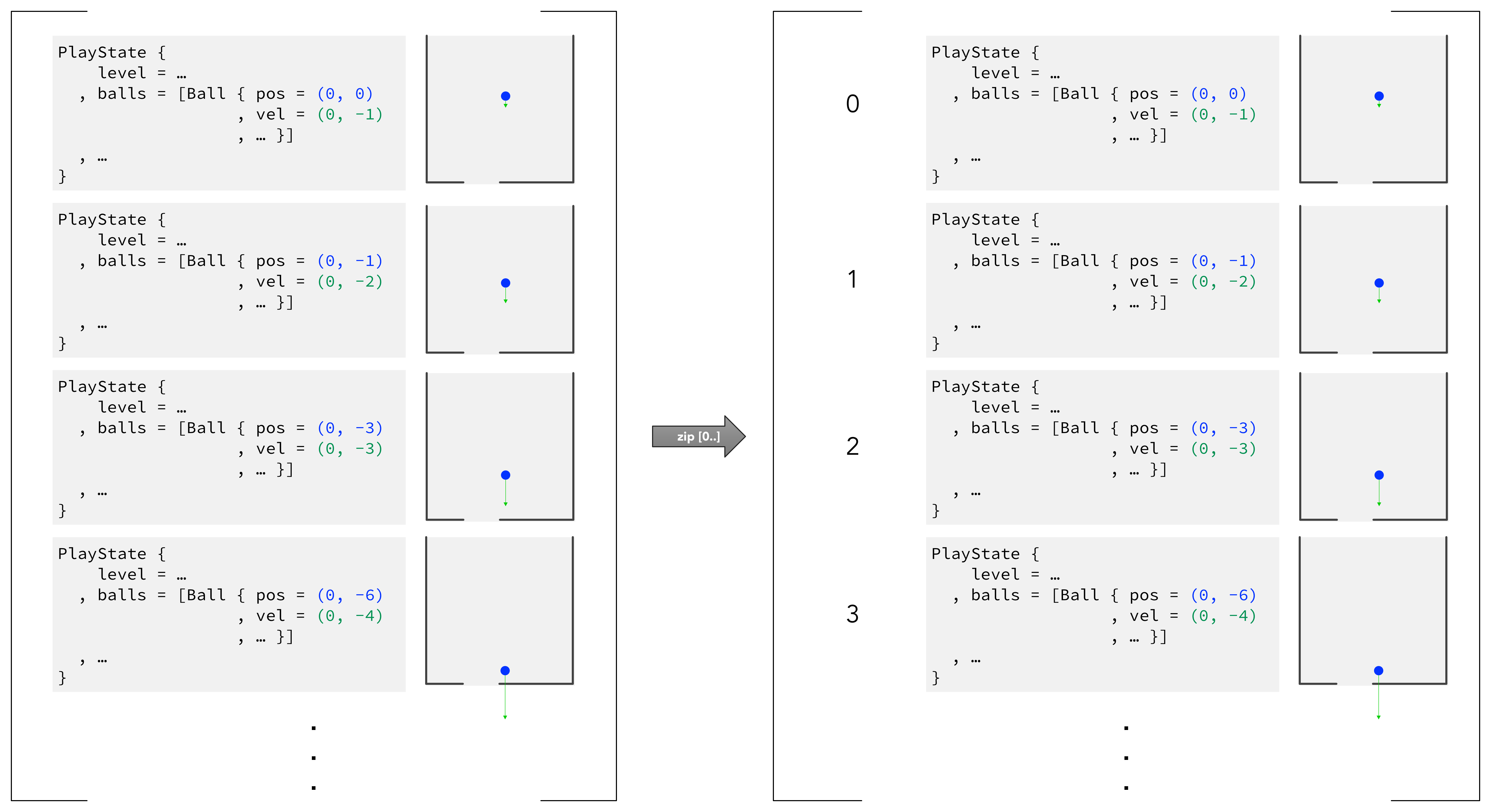
Zipping indices onto our predicted frames (enlarge)
-
filter: filter those future PlayStatesa.
fst: by looking at whether each PlayState's indexb.
(`mod` 15): mod 15c.
(== 0): is equal to 0. In other words, take every fifteenth frame from the listiterategave us.Now we have
[(0,the PlayState right now), (15,the PlayState 15 frames from now), (30,the PlayState 30 frames from now)...]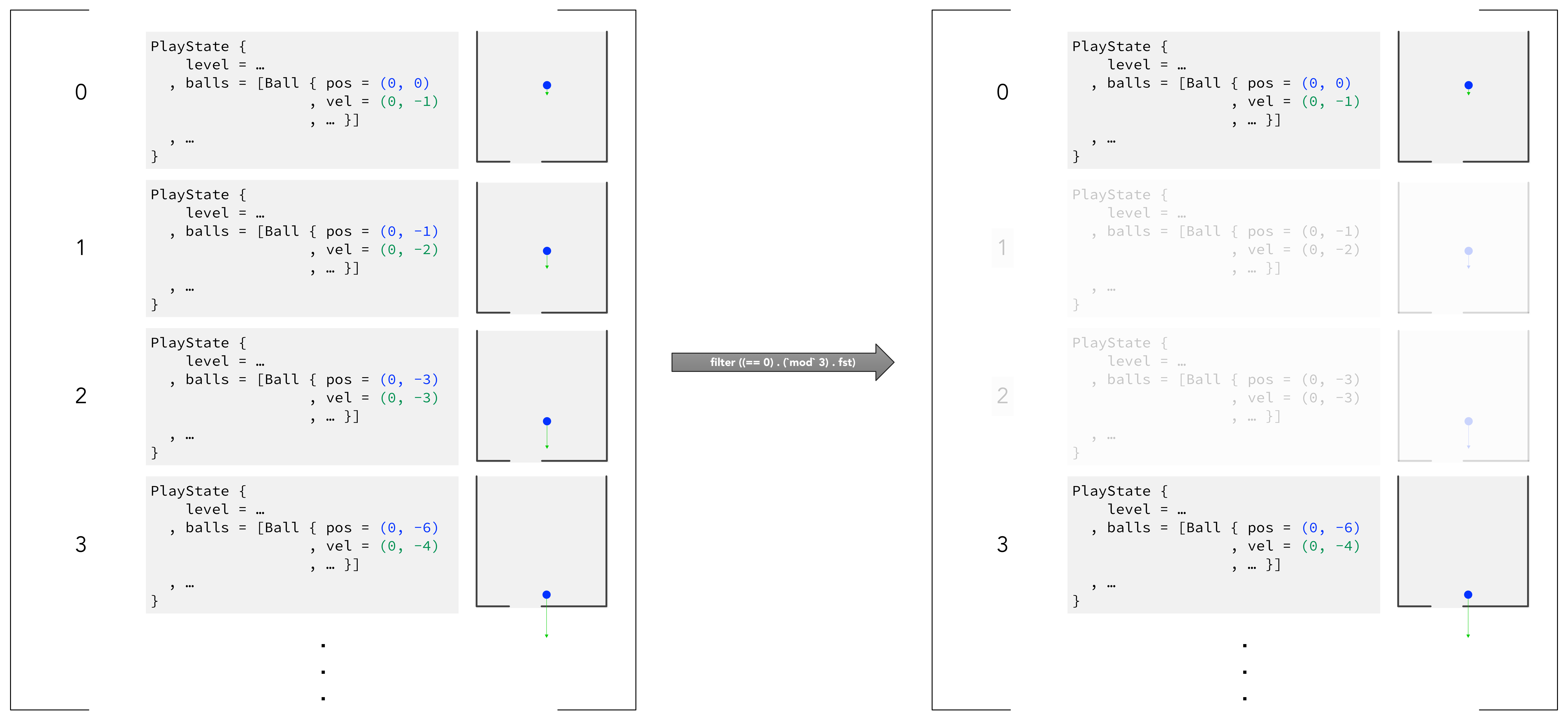
Filtering our infinite list so that we only take every third frame (I use mod 3 instead of mod 15 here to make it easier to see) (enlarge)
-
map (drawFutureBalls 50000): We don't want to just usedrawPlayStateand redraw the walls and everything, so we have a simple helper functiondrawFutureBallswhich just draws the ball from a PlayState, and grays it out depending on how far into the future it is (using the index tags fromzip). The 50000 parameter is sort of the 'denominator' of the graying function.At this point, we have a list of pictures of the ball in future frames:
[Picture of the ball right now,Picture of the ball 15 frames from now (grayed out a little),Picture of the ball 30 frames from now (even more grayed out)...]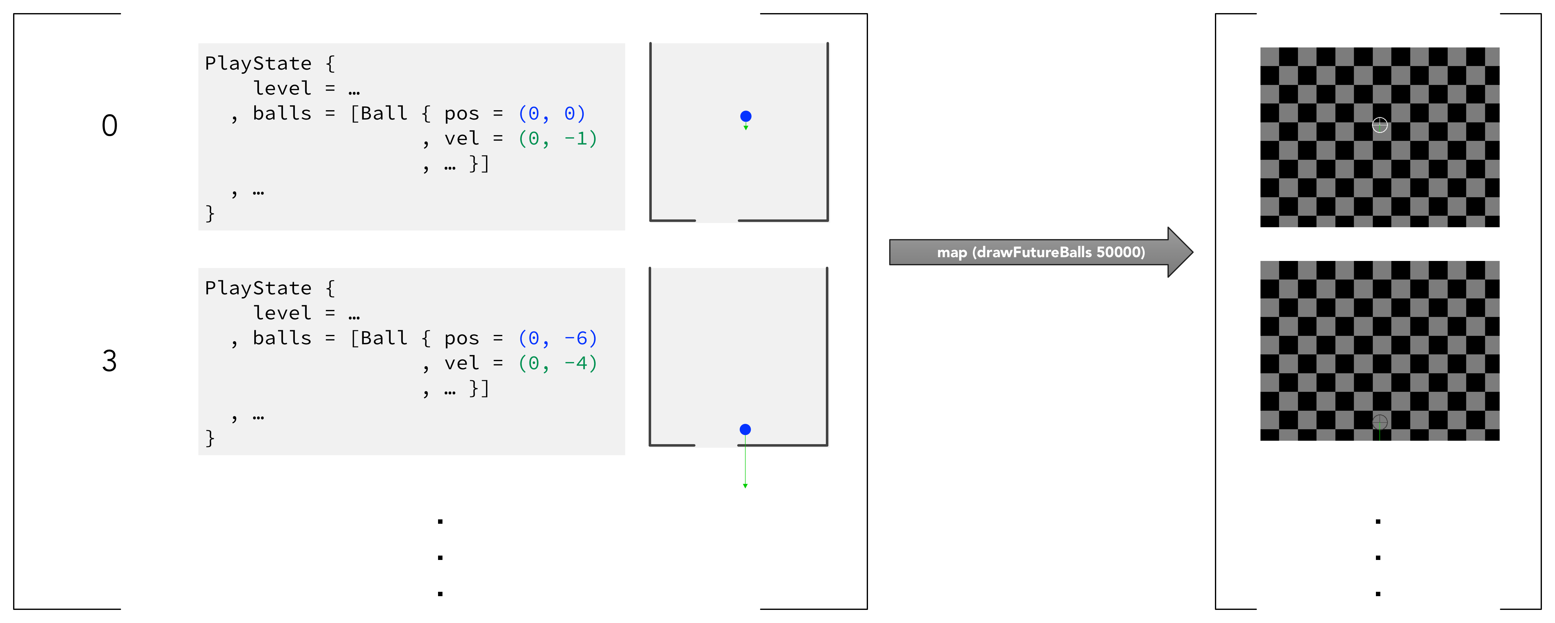
Turning PlayState data into pictures of future balls (enlarge). Note that the checkered background of the pictures (right) indicates that they have transparent backgrounds.
-
take 100: We don't want to render an infinite list of pictures, so let's just take the first 100 of the frames in our list. The higher the number we give here, the longer the ball's 'future trail' will extend.7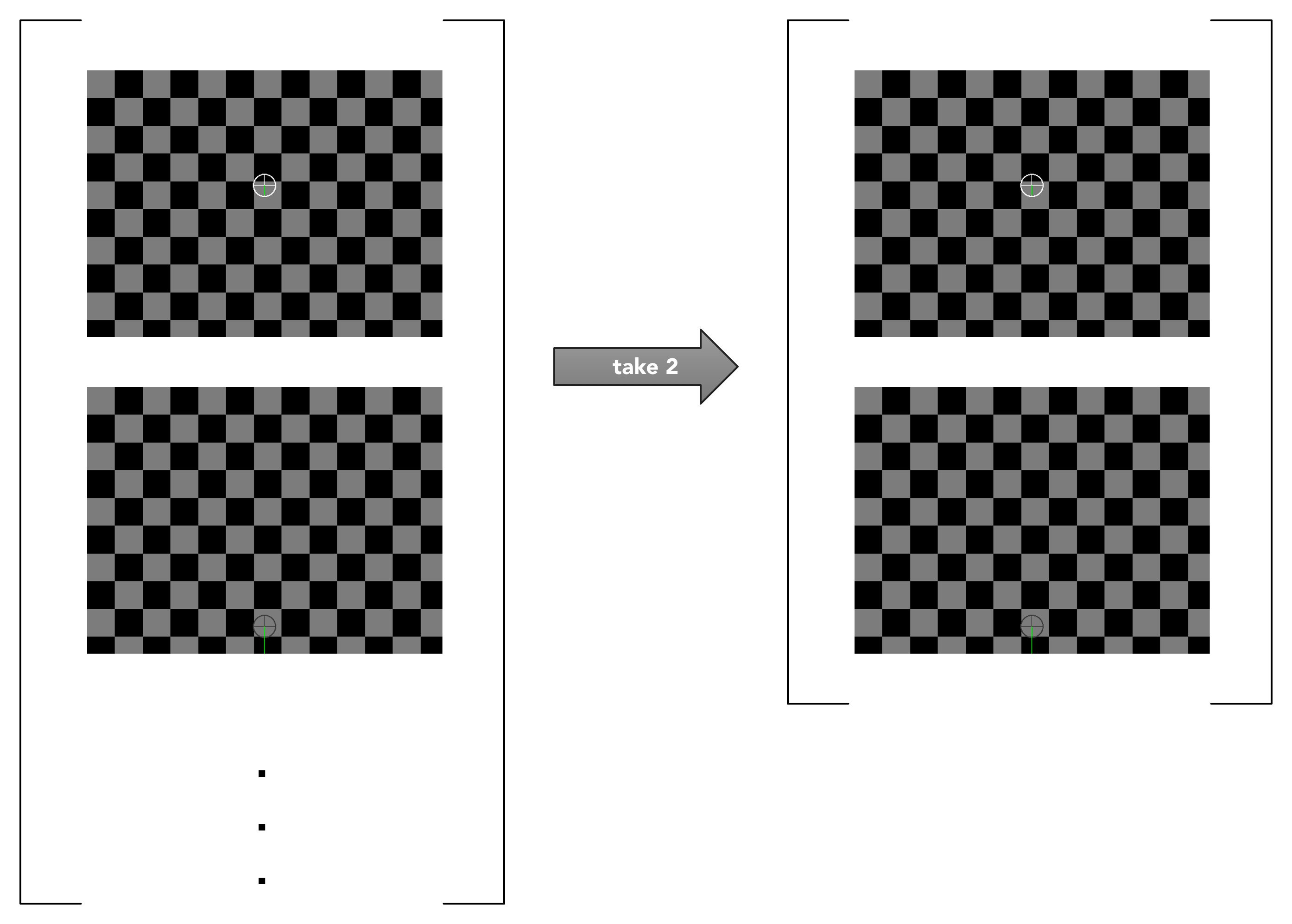
Taking a finite number of picture frames from the infinite list of frames (enlarge). Again, I've simplified from
take 100totake 2to make the effect easier to see.
-
pictures: Overlay all 100 frames in the[Picture]list that we've accumulated (like transparencies put on top of each other), resulting in one Picture that we can send back todrawPlayfor rendering.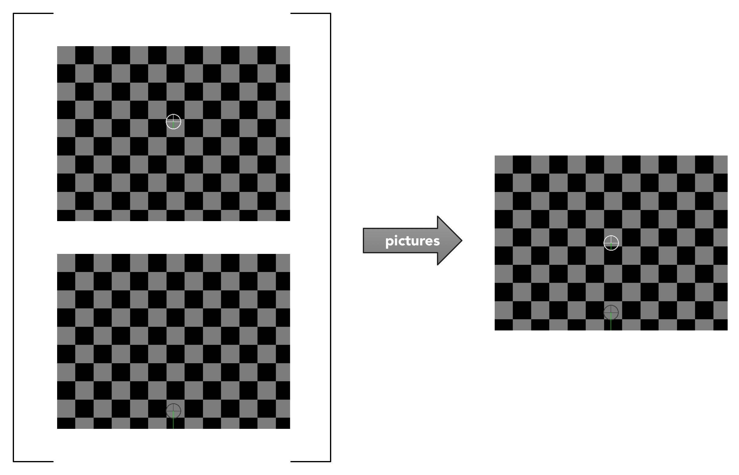
Combining all our frames (enlarge)
The entire pipeline (enlarge)
The playing around we did with sampling resolution in the last section is straightforward to explain now: first do take 1000 instead of take 100 to see further out, and then do mod 1 instead of mod 15 (or, better yet, remove the filter entirely) to get a smoother, higher-resolution curve; you're viewing every frame instead of every fifteenth frame.
Filtering with mod 15 (left) vs. mod 1 (right)
Again, it was representing our state transition from frame to frame as a pure function that made this 'seeing into the future' business so easy.8
Conclusions
I'd been planning to turn this demo into a more substantial game, but I haven't gotten around to it. I left off in May of last year, halfway through writing a level editor.
Over the past few days, I did set up a 'minimum viable' level system so I could compare the same situation across different builds (as you can see in the first section).
You can press S ingame to save the lines you've drawn as a .pinhole (plain-text JSON) file in a Pinhole folder (inside your home or Documents folder).
To load a level, you can drag the level file onto the program in Windows (or name your level of choice 'level.pinhole' and put it in your Pinhole folder [where saves go] on Windows or Mac OS). If you edit the level file manually in Notepad, I can't guarantee that it'll do the right thing, but you might be able to do some neat stuff.
A level file (enlarge). It lists five walls: I drew one ingame, and the four others are actually the default walls on the left, right, and bottom edges of the screen.
I also wrote the physics simulation from scratch, which was an interesting experience. (It's just one file.) I still sometimes think I can glimpse some slippage in the ball's rolling. There's a really cool physics bug you'll encounter in the demo that I never bothered to fix---you'll know it when you see it; you'll feel like you're playing with a yo-yo.
I was subconsciously influenced here by Bret Victor's Up and Down the Ladder of Abstraction and consciously influenced by the first example in his Inventing on Principle. I'm not sure where my demo falls between 'fun' and 'learning' (if such a spectrum does exist); I'm a little more interested in fun right now, and I think the high responsiveness of the demo makes it enormously satisfying to play with, even though it's got no real higher-level goals.
One intriguing idea this demo seems to suggest is games where state is visible instead of hidden---where the game goes out of its way to tell you exactly what's going on at all times, and it's clear exactly what the consequences of your actions are, but you get challenged in some different way.
Though not a full game, it's a fun demo to play around with. Give it a try!
You can reach me by e-mail or follow me on Twitter at @rsnous to keep track of what I'm up to. I'd love to hear about bug reports, level suggestions, levels, other places where these ideas could be cool, and anything else you have to say.
-
Software you have to download! Isn't that quaint? That's my biggest problem with choosing these tools. (But this might be a bias because I come from Web development; Unity seems to be doing OK.) The GHCJS project should eventually compile this thing into a Web app; Luite Stegeman actually ported the exact graphics and game library I'm using, Gloss, so that basic examples would render to a canvas in a browser. But that specific library port hasn't been polished up or officially released, and the code GHCJS generates is supposed to be huge. ↩︎
- The scaling of the green segment is a little fudged. But it does tell you the *direction* of the ball's velocity, and it's useful for comparing the velocity's magnitude between frames, at least. ↩︎
-
I wonder what equation describes that curve? ↩︎
-
Arbitrarily chosen numbers. I just picked whatever made the rolling look OK with my physics simulation functions. ↩︎
-
The `docState` and `drawing` fields are particularly interesting. I've been thinking about how writing functional user interfaces and games encourages you to see the 'state machines' underlying many of our interactions with the computer. Drawing a line is an example: you're either not drawing or drawing, and there are specific ways to transition from one state to the other (you put your mouse down, you lift your mouse up). The [sum type](https://en.wikipedia.org/wiki/Sum_type) directly represents the possible states of the system.
But the states may also have variables attached---the point where you started drawing and the point where you're at now, if you're drawing a line. Wikipedia says this kind of machine is an [extended state machine](https://en.wikipedia.org/wiki/UML_state_machine#Extended_states), in sort of a UML and flowchart tradition, but that doesn't seem satisfying as a formalism.
Drag and drop is a similar situation. Let's imagine the transitions are independent from state variables (a state variable would be data embedded in a state, something like 'the data the user's dragging' or 'the coordinates where the drag started'). Then we pretty much have an ordinary finite state machine ([enlarge](images/dragAndDrop.png)):
↩︎
-
https://en.wikipedia.org/wiki/Nineteen_Eighty-Four#Futurology ↩︎
-
Remember, we're sampling every 15 frames, so we are really taking a sample of the next 1500 frames. The demo runs at 60 frames per second, so we're visualizing about (1500 / 60) = 25 seconds into the future. ↩︎
-
If we were using Java, we might have a PlayState object with some methods that update private member variables in place, in the object, each frame. That design would work fine for just playing the demo, but every frame, we'd need to go out of our way to clone that object for *every predicted frame* to do anything cool like we did here. Otherwise, you'd overwrite your real PlayState with your predictions, and you wouldn't be able to actually play the demo.
I would never claim that, on the basis of this project, Haskell is an unequivocally better language than X mainstream language, or that you should switch your hairy enterprise system over just because this demo worked out well.
I do want to give some concrete evidence that it can be a powerful tool for creative play and programming on a similar scale to this demo, and I believe this example is more compelling than a one-liner. In fact, [John Carmack](https://en.wikipedia.org/wiki/John_D._Carmack), in his [exploration of Haskell](http://functionaltalks.org/2013/08/26/john-carmack-thoughts-on-haskell/) (see 17:40--22:18), envisioned a similar architecture to Gloss's (at bigger scale, with multiple entities), with a static state of the world that you transform into a new and separate state of the world.
↩︎